System Identification and Data Analysis
Contents of the course
The goal of this course is to introduce various methods to infer mathematical models from empirical observations. We will explore four subjects:
-
 The least squares method.
This is a cornerstone of applied mathematics, developed by Gauss
at the beginning of the 19th century; every engineer should be familiar with it,
and be ready to apply it as a general-purpose approximation method.
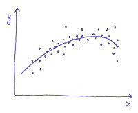
The goal of this method is to find,
in a family of functions indexed by a "parameter", the function (= the "parameter") that
provides the best description of a set of data (xi, yi), where
yi is supposed to be a function of xi plus some noise, and where
"best" means that the function chosen by the method minimizes the sum of squares of the approximation errors.
Such function can be useful, in particular, to predict the behavior of future data,
or also as an indirect way to measure the "parameter", in case the latter has a physical
interpretation but is not directly accessible.
We will show that the solution to this problem is readily computable
whenever the dependence on the "parameter" is linear (this is often the case
in practical applications), that the solution enjoys nice
statistical properties, and how the method can be applied
in a straightforward way to the identification of certain classes of
discrete-time linear dynamical models.
The least squares method.
This is a cornerstone of applied mathematics, developed by Gauss
at the beginning of the 19th century; every engineer should be familiar with it,
and be ready to apply it as a general-purpose approximation method.
The goal of this method is to find,
in a family of functions indexed by a "parameter", the function (= the "parameter") that
provides the best description of a set of data (xi, yi), where
yi is supposed to be a function of xi plus some noise, and where
"best" means that the function chosen by the method minimizes the sum of squares of the approximation errors.
Such function can be useful, in particular, to predict the behavior of future data,
or also as an indirect way to measure the "parameter", in case the latter has a physical
interpretation but is not directly accessible.
We will show that the solution to this problem is readily computable
whenever the dependence on the "parameter" is linear (this is often the case
in practical applications), that the solution enjoys nice
statistical properties, and how the method can be applied
in a straightforward way to the identification of certain classes of
discrete-time linear dynamical models.
-
 The LSCR (Leave-out Sign-dominant Correlation Regions) method.
The least squares method allows one to find the estimate of
a certain "true" parameter, that is, a "point" in Rp.
Despite the fact that in the limit (when the number of
data tends to infinity) the estimate converges to the "true" parameter,
no probabilistic guarantees can be given for the least squares solution with finite data,
unless strong assumptions are made on the law that generates them.
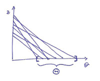
The LSCR method is designed to overcome this difficulty; its goal
is to find a confidence region of Rp in which the "true" parameter
lies with a certified probability, irrespective of the distribution
of the noise that corrupts the data.
The method is a recent development, in particular due to Marco Campi (University of Brescia)
and Erik Weyer (University of Melbourne, Australia).
The LSCR (Leave-out Sign-dominant Correlation Regions) method.
The least squares method allows one to find the estimate of
a certain "true" parameter, that is, a "point" in Rp.
Despite the fact that in the limit (when the number of
data tends to infinity) the estimate converges to the "true" parameter,
no probabilistic guarantees can be given for the least squares solution with finite data,
unless strong assumptions are made on the law that generates them.
The LSCR method is designed to overcome this difficulty; its goal
is to find a confidence region of Rp in which the "true" parameter
lies with a certified probability, irrespective of the distribution
of the noise that corrupts the data.
The method is a recent development, in particular due to Marco Campi (University of Brescia)
and Erik Weyer (University of Melbourne, Australia).
-
 Interval predictor models.
This is also a recent development, in particular due to Marco Campi,
Giuseppe Calafiore (Politecnico di Torino), and Simone Garatti (Politecnico di Milano).
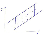
The ultimate goal of this method, alike the least squares method,
is to predict the behavior of future data. In this case, though, the estimate
will not come in the form of a function, fitted to the past data, that is supposed
to map a future independent variable x to a
prediction of the future dependent variable y; instead, the method will yield a function
that maps a future x to an entire interval which, with certified probability, will
contain the future y.
In particular, the computation of such an "interval predictor" relies on the solution of
a convex optimization problem, and the probabilistic guarantee comes from a clever application
of a deep result in geometry, Helly's theorem.
Interval predictor models.
This is also a recent development, in particular due to Marco Campi,
Giuseppe Calafiore (Politecnico di Torino), and Simone Garatti (Politecnico di Milano).
The ultimate goal of this method, alike the least squares method,
is to predict the behavior of future data. In this case, though, the estimate
will not come in the form of a function, fitted to the past data, that is supposed
to map a future independent variable x to a
prediction of the future dependent variable y; instead, the method will yield a function
that maps a future x to an entire interval which, with certified probability, will
contain the future y.
In particular, the computation of such an "interval predictor" relies on the solution of
a convex optimization problem, and the probabilistic guarantee comes from a clever application
of a deep result in geometry, Helly's theorem.
-
 Machine learning.
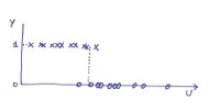
In this part of the course we will introduce classification problems,
focus on binary classification applied to simple models, and relate
the empirical classification error (the proportion of errors over the training set)
to the true error (the probability of error on yet unseen data).
In doing so, we will explore some classical and fundamental results in
non-parametric statistics, notably the theorem of Glivenko and Cantelli.
The goal of this part of the course is not really to provide off-the-shelf
methods that can be readily applied
(as may be the case for the other three parts), but to
understand with very simple examples the intrinsic limits in the art
of learning from empirical data.
Machine learning.
In this part of the course we will introduce classification problems,
focus on binary classification applied to simple models, and relate
the empirical classification error (the proportion of errors over the training set)
to the true error (the probability of error on yet unseen data).
In doing so, we will explore some classical and fundamental results in
non-parametric statistics, notably the theorem of Glivenko and Cantelli.
The goal of this part of the course is not really to provide off-the-shelf
methods that can be readily applied
(as may be the case for the other three parts), but to
understand with very simple examples the intrinsic limits in the art
of learning from empirical data.
All these subjects will be illustrated with practical examples. Possibly, the course will be integrated with seminars on real applications, given by members of our research group. Finally, if there is enough time, we will investigate in more depth the algebraic aspects of the least squares method, with a fast-paced introduction to the so-called Moore-Penrose pseudoinverse.
Prerequisites
The prerequisite of the course is a working knowledge of calculus, linear algebra, and probability theory; some results which are not usually taught in basic courses will be reviewed when needed.
Logistics for Spring 2017
The course will be taught in English.
The lecture schedule is as follows:| Day | Time | Place |
|---|---|---|
| Thursday | 15:30 - 18:30 | Room B1.5 |
| Friday | 11:30 - 13:30 | Room B1.5 |
Office hours are scheduled on Friday afternoon, in my office (please send an email before). But if you attend the course and you want to discuss the material seen in class or ask questions, we can arrange other meetings as well.
The examination will be written (no books or notes allowed) and oral, at fixed sessions. The written test will be in English, and the oral examination will be in English or Italian, at your choice.
Here are the instructions regarding the written tests.
Learning material
| File | Comments |
|---|---|
| sida.pdf | These are the lecture notes for the course. Please understand that they are still a work in progress. If you spot errors or if you have other suggestions, please send me an email. |
| problems.pdf | A set of exercises with solutions. The exercises are also at the end of the respective chapters in the lecture notes, and the solutions in an appendix. This document is also a work in progress. |
| Insane correlations | "There is a 95% correlation between this and that, hence we have strong statistical evidence that..." Have a look at this page before you even dream of completing the sentence! |
| (youtube video) | Review of Linear Algebra 1 (ca. 50 minutes): MIT 18.085 Computational Science and Engineering I, Fall 2008 Recitation 1, by prof. Gilbert Strang. MIT OpenCourseWare, © The Massachusetts Institute of Technology. |
| (youtube video) | Review of Linear Algebra 2 (ca. 60 minutes): MIT 18.085 Computational Science and Engineering Lecture 1, by prof. Gilbert Strang.
MIT OpenCourseWare, © The Massachusetts Institute of Technology. (This and the previous link point to lectures from two different editions of the same course, delivered by one of the best teachers in the world. Needless to say, you would gain a lot by watching other lectures of that course, although they are not necessarily related to our S.I.D.A. course.) |
| lscode.zip | Matlab/Octave code for Chapter 1 (exercises on least squares). |
| idcode.zip | Matlab/Octave code for Chapter 3 (ARX identification/instrumental variables). |
| (link to paper) | George Udny Yule, On a Method of Investigating Periodicities in Disturbed Series, with Special Reference to Wolfer's Sunspot Numbers, Philosophical Transactions of the Royal Society of London, 1927. |
| sunspots.zip | Matlab/Octave and R code: AR(2) fit of Wolf's sunspot numbers, as in Yule's paper. |
| nllscode.zip | Matlab/Octave code for Chapter 4 (Levenberg-Marquardt method and examples). |
| glivenko_cantelli.m | Matlab/Octave code: test of the Glivenko/Cantelli theorem. |
In general, the above lecture notes will be sufficient for the course's purposes. Nevertheless, the good-willing student (also known as you) is of course welcome to refer to other sources as well. A standard textbook that covers in full generality classical and modern aspects of system identification is
- L. Ljung. System Identification - Theory for the user, 2nd ed. Prentice-Hall.
For the sections regarding LSCR and the Interval Predictor Models, which are recent developments, the interested student can also refer to the following original research papers (they cover the respective subjects in far more depth than we will do in class):