Data Driven System Modelling
Contents of the course
-
 Fitting data with models.
This course is about finding mathematical models to fit empirical data coming from
measures (e.g. from engineering applications, econometric time series, statistical surveys, and so on.).
To fix ideas, think of a series of input-output pairs (xi, yi).
The first steps will be to understand what a mathematical model actually is
(in the simplest case, just a real-valued function mapping input to output: y = f(x)), to distinguish between
static models versus dynamical ones,
to justify the main goal of fitting (typically prediction of future observations: ypredicted = f(xfuture)),
and to justify the need for a reasonable model class:
indeed, in no way one can start the fitting endeavour from "no knowledge at all", or s/he will immediately
find him/herself disoriented by the immense complexity of the set of "all the possible models" (whatever this may mean),
get lost in the swamp of non-uniqueness, and almost surely obtain a completely useless model.
No: the experimenter must start from a "theory", i.e. from a restricted
and sufficiently simple set of models, coming from past experience, scientific laws, or just common sense.
Fitting data with models.
This course is about finding mathematical models to fit empirical data coming from
measures (e.g. from engineering applications, econometric time series, statistical surveys, and so on.).
To fix ideas, think of a series of input-output pairs (xi, yi).
The first steps will be to understand what a mathematical model actually is
(in the simplest case, just a real-valued function mapping input to output: y = f(x)), to distinguish between
static models versus dynamical ones,
to justify the main goal of fitting (typically prediction of future observations: ypredicted = f(xfuture)),
and to justify the need for a reasonable model class:
indeed, in no way one can start the fitting endeavour from "no knowledge at all", or s/he will immediately
find him/herself disoriented by the immense complexity of the set of "all the possible models" (whatever this may mean),
get lost in the swamp of non-uniqueness, and almost surely obtain a completely useless model.
No: the experimenter must start from a "theory", i.e. from a restricted
and sufficiently simple set of models, coming from past experience, scientific laws, or just common sense.
Visualize: to fit a collection of noisy measures (vt, it), where vt and it are respectively a voltage and a current across a resistor at given times t = t1, t2, t3, ..., you don't have to search among all possible functions v = f(i), for you already know Ohm's law. No no: it makes much more sense to choose the model among linear functions: v = Ri, where R > 0 is an unknown "parameter". The set of linear functions {f(i) = Ri | R > 0} is the model class: now the name of the game is to estimate R from the data.
We will explore the meaning of prediction: what does the model have to say about future measures, and in what sense(s) one can be confident about the provided information.
-
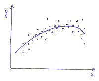
The least squares method.
This is a cornerstone of applied mathematics, developed by Gauss
at the beginning of the 19th century; every engineer should be familiar with it,
and be ready to apply it as a general-purpose approximation method.
The goal of this method is to find,
in a family of functions indexed by a "parameter", the function (= the "parameter") that
provides the best description of a set of data (xi, yi), where
yi is supposed to be a function of xi plus some noise, and where
"best" means that the function chosen by the method minimizes the sum of squares of the approximation errors.
We will show that the solution to this problem is readily computable
whenever the dependence on the "parameter" is linear (this is often the case
in practical applications).
We will show that, even when the model family is very large (read: the parameter lives in a high-dimensional space), we can fight against so-called "overfitting" by putting a cost on complexity (read: the effective number of "active" parameters), thus regularizing the problem; when the dependence on the parameter is linear the regularized problem is almost as simple as the standard one.
Finally, we will show that the method, besides providing a means to predict the behavior of future data, can be employed also as an indirect way to measure a hidden "true parameter", when the latter has a physical interpretation but is not directly accessible. In this way the LS method, which is algorithmic in nature, enters the realm of statistical estimation: we will explore how the estimation from input-output pairs depends crucially on the information contained in the input record, introduce notions of "goodness" of an estimator, and show why the LS solution, under fairly general hypotheses, enjoys many of them.
-
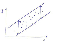 Interval predictor models.
This is a recent development, in particular due to Marco Campi,
Giuseppe Calafiore (Politecnico di Torino), and Simone Garatti (Politecnico di Milano).
The ultimate goal of this method, alike the least squares method,
is to predict the behavior of future data. In this case, though, the estimate
will not come in the form of a function, fitted to the past data, that is supposed
to map a future independent variable x to a
prediction of the future dependent variable y; instead, the method will yield a function
that maps a future x to an entire interval which, with certified probability, will
contain the future y.
In particular, the computation of such an "interval predictor" relies on the solution of
a convex optimization problem, and the probabilistic guarantee comes from a clever application
of a deep result in geometry, Helly's theorem.
Both Least Squares and the method of Interval Predictor Model are forms of what in statistics is called
regression: we will see how both of them (and other regression methods) can be
interpreted geometrically as the minimization of a distance.
Interval predictor models.
This is a recent development, in particular due to Marco Campi,
Giuseppe Calafiore (Politecnico di Torino), and Simone Garatti (Politecnico di Milano).
The ultimate goal of this method, alike the least squares method,
is to predict the behavior of future data. In this case, though, the estimate
will not come in the form of a function, fitted to the past data, that is supposed
to map a future independent variable x to a
prediction of the future dependent variable y; instead, the method will yield a function
that maps a future x to an entire interval which, with certified probability, will
contain the future y.
In particular, the computation of such an "interval predictor" relies on the solution of
a convex optimization problem, and the probabilistic guarantee comes from a clever application
of a deep result in geometry, Helly's theorem.
Both Least Squares and the method of Interval Predictor Model are forms of what in statistics is called
regression: we will see how both of them (and other regression methods) can be
interpreted geometrically as the minimization of a distance.
-
Dynamical models, prediction theory, and system identification.
Armed with regression methods, we will study the problem of identifying dynamical
models, i.e. mathematical models suitable to describe phenomena where forces are
involved or, in abstract terms, phenomena whose output depends not just on the istantaneous
input, but also on the past behavior of the input and the output. To fix ideas: a resistor
is well described by a static model v = Ri, but a RC network does not: it needs a dynamical
model, that in continuous time typically takes the form of a differential equation.
We will always work in discrete time. This is well justified on one hand by the fact that differential equations can be discretized with good approximation (continuous signals can be sampled), and on the other hand by the fact that identification and its applications (control) are now done by means of digital computers, that work in discrete time by definition. In information engineering, fitting a time series of data with a dynamical model is called system identification, and the general method that extends Least Squares to system identification is called Prediction Error Minimization (PEM).
We will explore model classes best suited to represent discretizations of linear differential equations; these are called difference equations, fall under different names (AR, MA, ARMA, ARX, ARMAX, ...) depending on their structure, and pose different identification challenges: some of them involve an easy application of the ordinary Least Squares method; others do not, and require numerical non-convex optimization. The analysis of the kind of data that can be generated by a (stable) dynamical model and that of the statistical properties of the PEM will involve a tour in the theory of wide-sense stationary processes, prediction theory (a particular case of the so-called Wiener filter) and spectral analysis. Depending on the statistical behavior of the observed data, non-identifiability issues may arise: we will introduce alternative ways to carry on with identification (e.g. instrumental variables). We will explore the consequences (and the possible dangers) of doing system identification in closed loop. The course will end with the study of system identification in the frequency domain.
All these subjects will be illustrated with practical examples. Exercise classes will provide an introduction to standard system identification software (in Matlab/Octave, Python or R, depending on the context). Possibly, the course will be integrated with seminars on real applications, given by members of our research group. Finally, if there is enough time, we will investigate in more depth the algebraic aspects of the least squares method with a fast-paced introduction to the so-called Moore-Penrose pseudoinverse, and/or with the introduction to the Levenberg-Marquardt algorithm, a standard method for solving nonconvex least squares problems.
Prerequisites
The prerequisite of the course is a working knowledge of calculus, linear algebra, and probability theory; prior exposition to a course in signals and systems will be very useful. Some results which are not usually taught in basic courses will be reviewed when needed.
Logistics for Fall 2021
The course will be taught in English. The lecture schedule is as follows:
| Day | Time | Place |
|---|---|---|
| Tuesday | 17:00 - 19:00 | Room M1 (via Valotti 9) |
| Wednesday | 16:00 - 19:00 | Room B2.4 (via Branze 43) |
Office hours will be scheduled during the first week. Anyway, if you attend the course and you want to discuss the material seen in class or ask questions, we can arrange other meetings as well.
I suspect that the first lectures will suffer from a transient
due to the requirement frontal lecturing + remote lecturing and the
planned change in technology (from Google Meet to MS Teams).
Please subscribe to the Moodle community for the latest news:
DDSM 2021/22
After-course meeting for questions, review, exercises
| Date | Time | Place |
|---|---|---|
| ? | ? | ? |
The exam will be written (no books or notes allowed) and oral, at fixed sessions. The written test will be in English, and the oral examination will be in English or Italian, at your choice.
To those who could not subscribe to the course: please send me an email before the written test to confirm your participation.
Learning material
| File | Comments |
|---|---|
| short_ddsm.pdf | Here you will soon find a "compact" and agile set of lecture notes for the course; they will be inserted and grown as the course goes on, week after week. In the meanwhile, you may refer to chapters 1 and 3 of the lecture notes below. |
| sida.pdf | These are the lecture notes of the old course, System Identification and Data Analysis. They cover only some subjects of this course (and other subjects that will not be taught), but for now Chapters 1, 3 and the Appendices will serve as a good start. If you spot errors or if you have other suggestions, please send me an email. |
| Insane correlations | "There is a 95% correlation between this and that, hence we have strong statistical evidence that..." Have a look at this page before you even dream of completing the sentence! |
| (youtube video) | Review of Linear Algebra 1 (ca. 50 minutes): MIT 18.085 Computational Science and Engineering I, Fall 2008 Recitation 1, by prof. Gilbert Strang. MIT OpenCourseWare, © The Massachusetts Institute of Technology. |
| (youtube video) | Review of Linear Algebra 2 (ca. 60 minutes): MIT 18.085 Computational Science and Engineering Lecture 1, by prof. Gilbert Strang.
MIT OpenCourseWare, © The Massachusetts Institute of Technology. (This and the previous link point to lectures from two different editions of the same course, delivered by one of the best teachers in the world. Needless to say, you would gain a lot by watching other lectures of that course, although they are not necessarily related to our course.) |
| lscode.zip | Matlab/Octave code: exercises on least squares. |
| constrained.zip | Matlab/Octave code: example of constrained least squares. |
| model_order.zip | Matlab/Octave code: examples on model order selection (polynomial interpolation) with FPE and regularization. |
| ar_predictor.m | Matlab/Octave code: optimal predictor of an AR(2) process and comparison with sub-optimal predictors.. |
| idcode.zip | Matlab/Octave code for ARX identification and instrumental variables. |
| yule.pdf | George Udny Yule, On a Method of Investigating Periodicities in Disturbed Series, with Special Reference to Wolfer's Sunspot Numbers, Philosophical Transactions of the Royal Society of London, 1927. |
| sunspots.zip | Matlab/Octave and R code: AR(2) fit of Wolf's sunspot numbers, as in Yule's paper. |
| nllscode.zip | Matlab/Octave code: Levenberg-Marquardt method and examples. |
In general, the material provided above will be sufficient for the course's purposes. Nevertheless, the good-willing student (informally known as you) is of course welcome to refer to other sources as well. A standard textbook that covers in full generality classical and modern aspects of system identification is
- L. Ljung. System Identification - Theory for the user, 2nd ed. Prentice-Hall.
Regarding the Interval Predictor Models method, which is a recent development, the interested student can also refer to the following original research paper (they cover the respective subjects in far more depth than we will do in class):
- M.C. Campi, G. Calafiore and S. Garatti. Interval Predictor Models: Identification and Reliability (available at this link on prof. Campi's webpage).